Access Latest NAV on Google Sheets

Tracking the latest NAV of your NPS fund in Google Sheets is straightforward. By using the IMPORTDATA function, you can pull real-time NAV data directly into your spreadsheet. Here's how to do it:

Step 1: Use the IMPORTDATA Function

Google Sheets offers the IMPORTDATA function, which allows you to fetch external data using a URL. This feature is perfect for tracking NPS NAV data.

=IMPORTDATA("https://npsnav.in/api/SchemeCode")

Replace SchemeCode with the actual code of the NPS fund you want to track.

List of all available NPS schemes can be accessed here.

Example:

=IMPORTDATA("https://npsnav.in/api/SM001001")

Step 2: Calculate the Value of Your NPS Portfolio

Once you have the current NAV, you can calculate the value of your NPS portfolio by multiplying the NAV by the number of units you hold.

Example Calculation:

=IMPORTDATA("https://npsnav.in/api/SchemeCode") * 268

Make sure you input the correct scheme code and the number of units you hold in that particular NPS fund.

Step 3: Ensure You Choose the Right Fund

There are multiple NPS schemes under various tiers and schemes. Ensure that you choose the right fund as per your portfolio. You can find the complete list of scheme codes here.

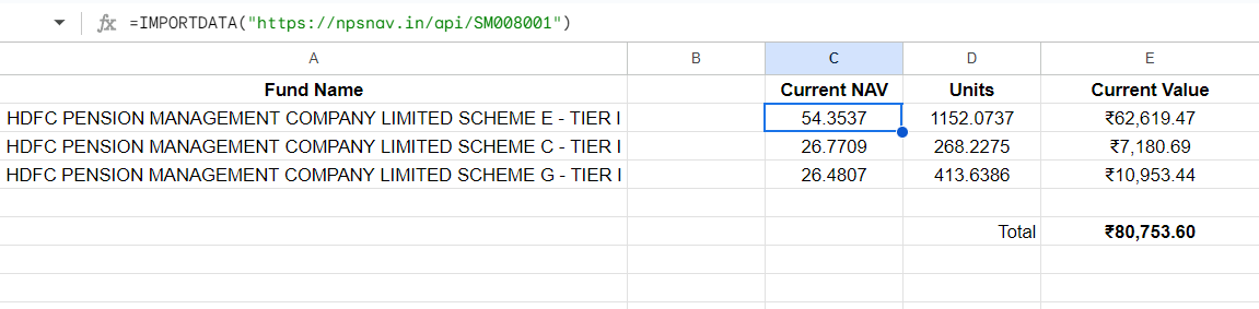
Example NPS Portfolio on Google Sheets

Below is an example screenshot of how a sample NPS portfolio looks on Google Sheets:

Access Historical NAV Data on Google Sheets

You can also fetch historical NAV data for any specific date using our historical API. This is useful for tracking performance over time or for reporting purposes.

Step 1: Set Up Your Input Cells

In cell A1, enter your scheme code (e.g., "SM010001")

In cell B1, enter your target date in a format Google Sheets recognizes as a date (e.g., "5/5/2025")

Step 2: Use the Historical API Formula

In another cell, enter this formula to get the NAV value for your target date:

=LET(
  import, IMPORTDATA("https://npsnav.in/api/historical/"&A1, ":"),
  dates, ARRAYFORMULA(VALUE(SUBSTITUTE(CHOOSECOLS(import,2), ",", ""))),
  INDEX(CHOOSECOLS(import,2), XMATCH(B1, dates, -1, 1)+1)
)

Step 3: Understand the Result

The formula will return the NAV value for the most recent date on or before your target date. If there was no NAV published exactly on your target date (such as weekends or holidays), it will show the last available NAV value.